Site grouping

For the analysis of emissions over a population of sites it is useful to be able to classify sites into a small number of groups. Almost every site is unique, with different characteristics and equipment. Without detailed equipment level data, both for emission sources and infrastructure itself, it is difficult to make statistical comparisons at the population level. By finding a natural classification for sites based on the properties of the available infrastructure data we are able to create more manageable sets of groups for comparison.

We will use a set of Bridger data that contains the counts of each equipment type on ~6000 sites. This gives us a seven dimensional parameter space in which to find clusters. However, trying to find sensible clusters of sites in such a high dimensional parameter space is difficult. Instead we want to extract the most meaningful components out of this seven dimensional parameter space and then cluster with respect to that. So we use a singular value decomposition to find what components are most important in terms of variability between sites. Then we fit clusters to this data and use the results to create a small set of site groups.

Singular value decomposition and clustering

In this section we briefly outline how a singular value decomposition (SVD) works. Given a real (or complex) matrix $A$ of dimensions $m\times n$, the SVD is a factorization of the form:

$$A=U\mathrm{\Sigma }{V}^T$$

Where:

• $A$ is the original $m\times n$ matrix.
• $U$ is an $m\times m$ orthogonal matrix (columns are the left singular vectors).
• $\mathrm{\Sigma }$ is an $m\times n$ diagonal matrix with non-negative real numbers on the diagonal (the singular values).
• $V$ is an $n\times n$ orthogonal matrix (columns are the right singular vectors).

The singular values ${\sigma }_i$ in $\mathrm{\Sigma }$ satisfy:

$${\sigma }_1\ge {\sigma }_2\ge \cdots \ge {\sigma }_r>0$$

Where $r=\text{rank}(A)$, and the remaining values (if any) are 0.

The singular values indicate the importance of each component in the factorization. Larger singular values correspond to components in the data with more variance, while smaller singular values contribute less. By discarding the smallest singular values, we can still closely approximate the original matrix, which is why SVD is so useful. It enables us to reduce the dimensionality of a dataset — for example, representing a site with many equipment types using only a few of the most significant features — while preserving most of the structure.

To determine the optimal number of components in the reduced matrix we can experiment and evaluate each component based on the values in $\mathrm{\Sigma }$. Once we have decomposed the original matrix into a smaller dimensional space, we can cluster sites into groups using the matrix $U$. Each row in this matrix still represents a site, but with less components. We then use K-means clustering to find the groups.

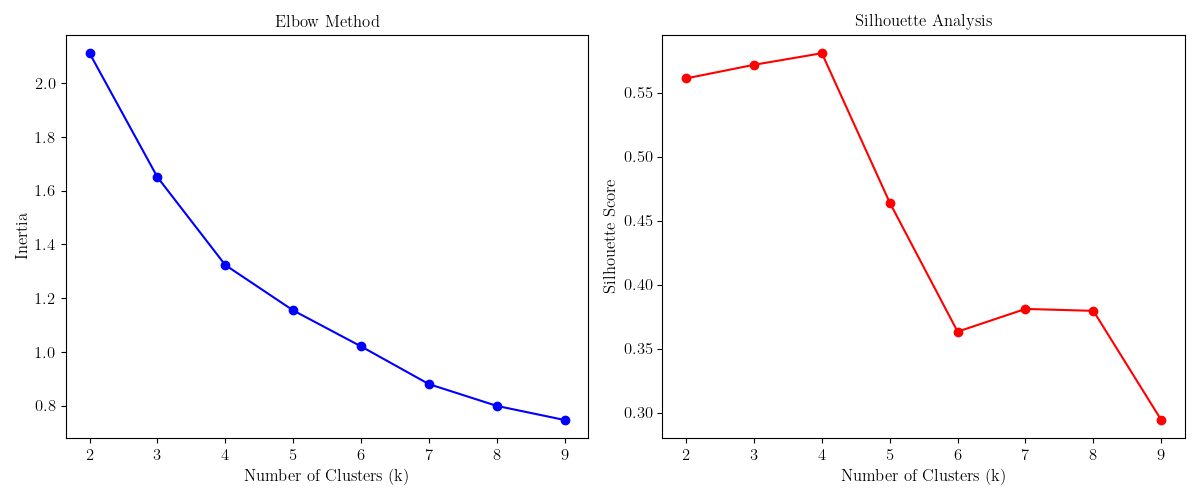
The number of clusters to aim for is based on a comparison of the quality across a set of choices. We use the "Elbow method" and "Silhouette analysis" to determine the optimal number of clusters.

Results for sites

We will use the following equipment counts from 6465 sites sourced from qf487 and vv144 Bridger surveys.

• Flare
• Tank
• Well
• Separator
• Compressor
• Generator
• VRU

Since the number of equipment items varies we normalise the counts by dividing by the median plus one (to account of types with a median of zero). We use the median as there are some outlier sites with very high counts of some equipment types that would skew the mean.

First we do a decomposition using five components, which gives us the relative strength of each, we find the following.

$$\mathrm{\Sigma }=\left[\begin{array}{ccccc}524.1& 0& 0& 0& 0\\ 0& 184.0& 0& 0& 0\\ 0& 0& 113.7& 0& 0\\ 0& 0& 0& 91.7& 0\\ 0& 0& 0& 0& 60.6\end{array}\right]$$

The number of components to include in our final decomposition is a matter of choice. If we use all components, it can be difficult to find good quality clusters of data in the higher dimensional parameter space - and would negate the point of doing an SVD. Instead, we choose a reasonable number of components to reduce down to, such that we can focus our clustering on the most important features.

Once a number of components has been selected we also need to determine how many clusters to use. Higher numbers of clusters result in lower inertia (a measure of spread within the cluster) but potential over fitting, that may work well for this dataset but does not capture the more general properties that would applicable to other sets of sites.

We see diminishing returns after three components, so we choose this as our number of dimensions. Further analysis (see the plots below) shows that fours clusters is also a good choice.

The groups are shown in the table below. The median number of each equipment type is given and in brackets we have the standard deviation.

Group	Count	Flare	Tank	Well	Separator	Compressor	Generator	VRU
0	745	2.0 (2.6)	11.0 (5.6)	2.0 (2.7)	4.0 (3.4)	0.0 (0.8)	0.0 (0.5)	0.0 (0.5)
1	7368	0.0 (0.7)	0.0 (2.0)	1.0 (1.4)	1.0 (2.0)	0.0 (0.5)	0.0 (0.2)	0.0 (0.4)
2	292	1.0 (1.1)	6.0 (7.8)	0.0 (2.3)	13.0 (9.0)	1.5 (2.4)	0.0 (0.7)	0.0 (2.3)
3	269	0.0 (3.8)	1.0 (6.0)	10.0 (7.1)	10.0 (9.2)	0.0 (0.9)	0.0 (0.2)	0.0 (0.3)

To make the site groups easier to understand we can classify the counts for the most important equipment types into low, medium and high values. This gives us the following simplified view.

Group	Count	Flare	Tank	Well	Separator	Compressor
0	745	High	High	Low	Medium	Low
1	7368	Low	Low	Low	Low	Low
2	292	Low	Medium	Low	High	High
3	269	Medium	Low	High	High	Low

So we have the following summary for each group.

• Group 0: Sites with the most tanks. Generally without compressors.
• Group 1: The most common, small sites. Generally without flares or compressors.
• Group 2: These sites have the most compressors and separators.
• Group 3: These sites have the most wells and a similar number of separators.

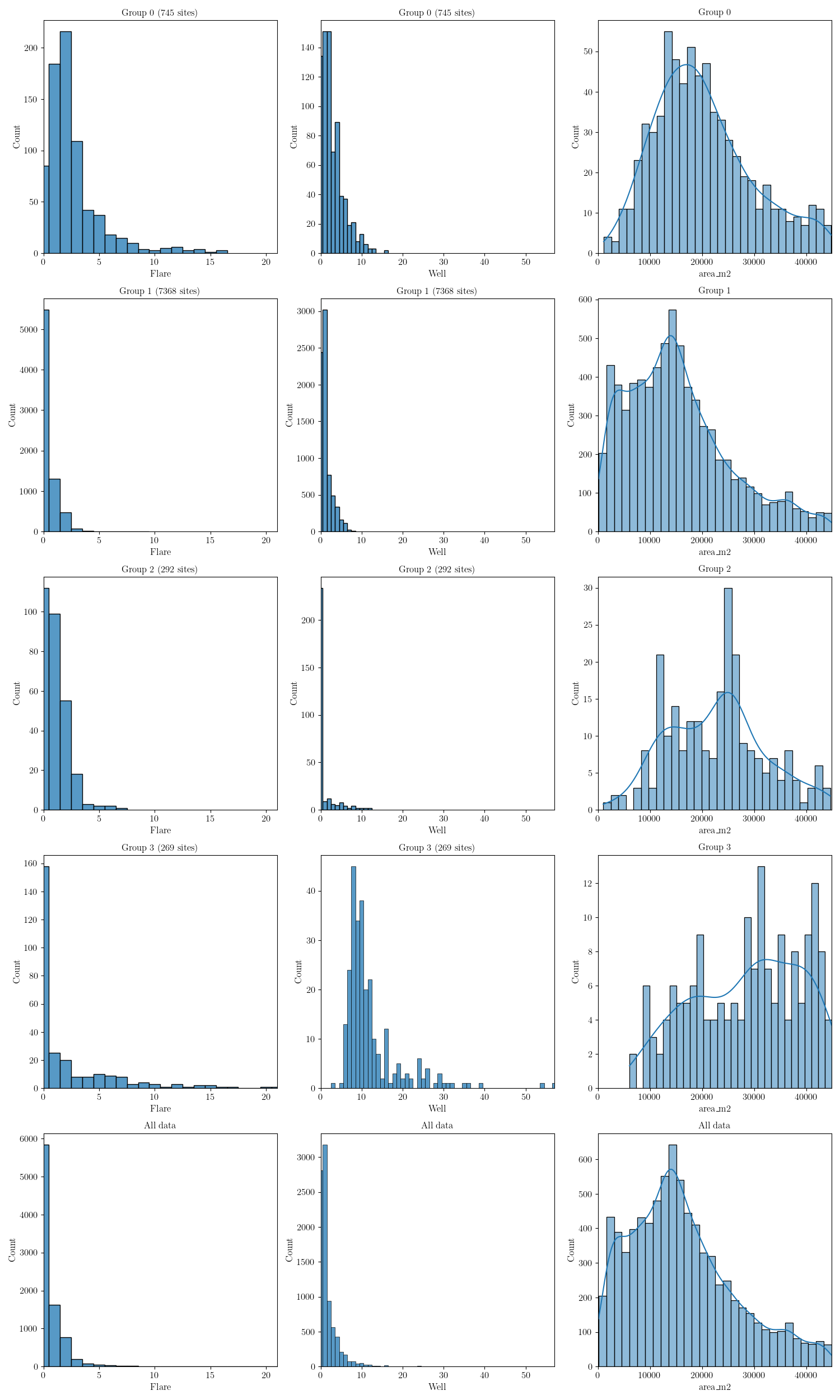
The figures below show the distribution of each equipment type across the groups. Since there are many components to consider we have three figures each containing the same information but for different equipment types. The first figure also shows the area. Note that this plot only shows up to a maximum of the 95th percentile, as there are some sites with very large areas which would make these plots difficult to interpret.

In the following figure we show flares and wells. We also include the area of the sites.

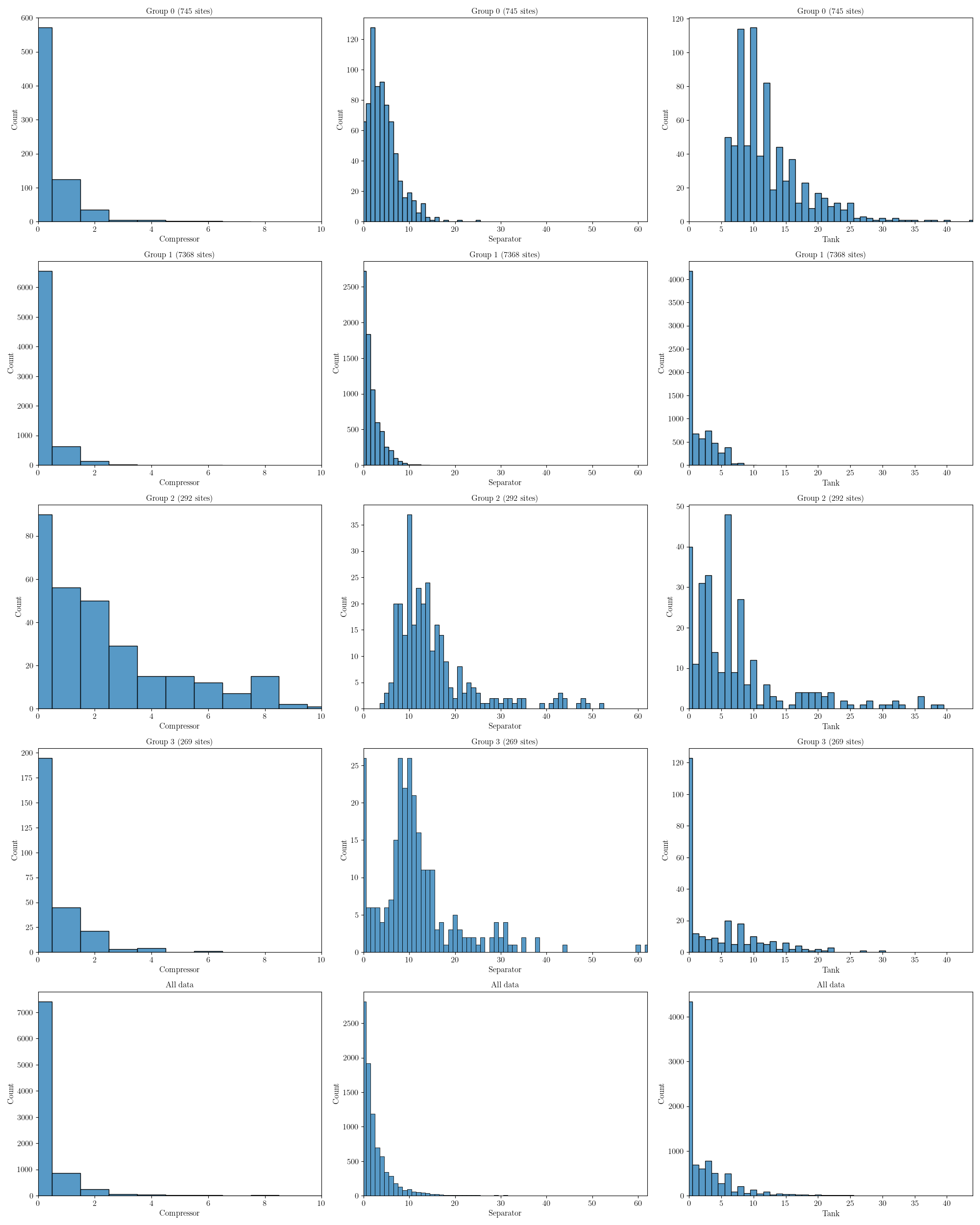
Below we show compressors, separators and tanks.

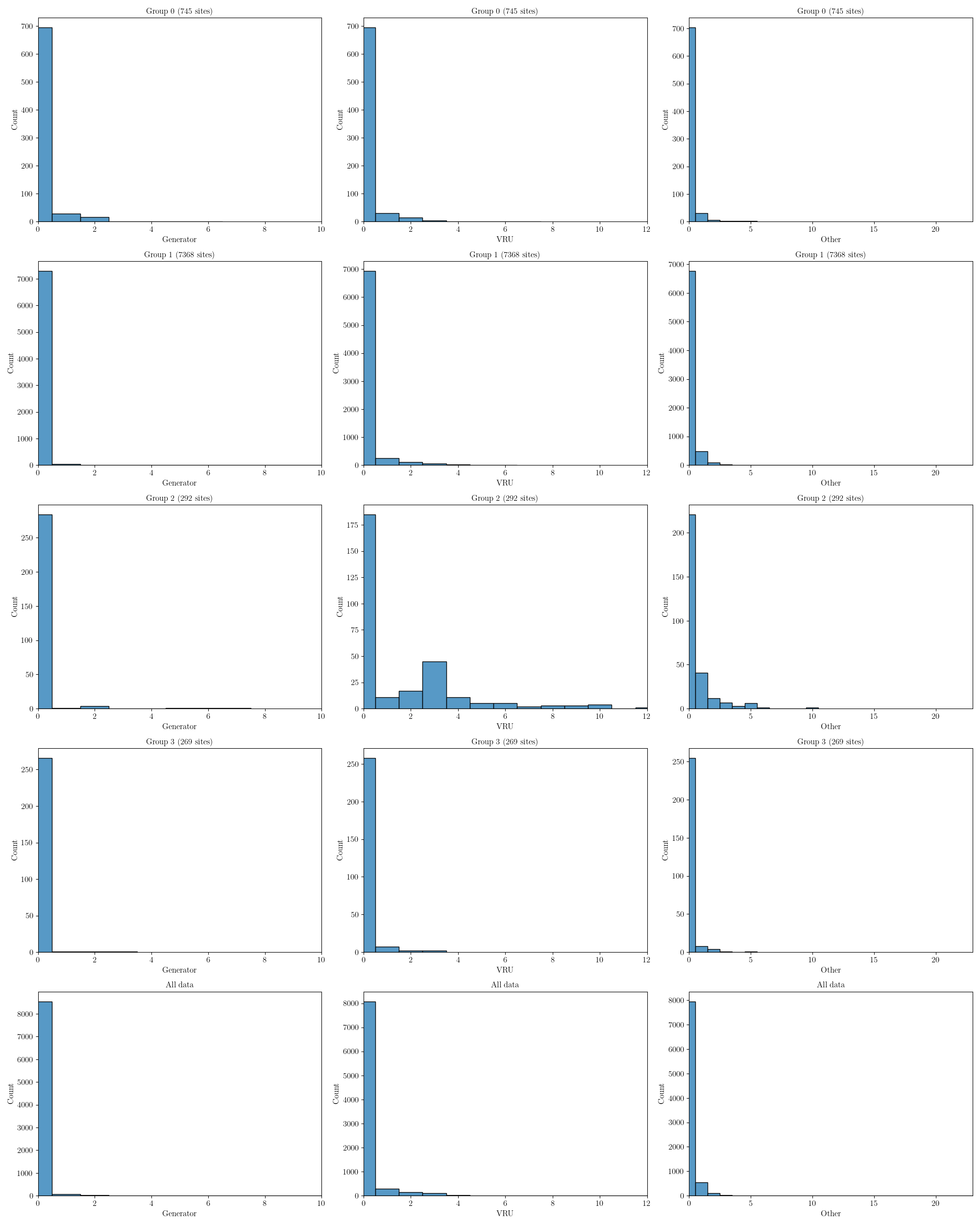
In the final figure we show generators, VRUs and the count of any other equipment (note that other is not included in the analysis at all, doing so leads to poor quality results).

The following figure shows the results of the "Elbow method" and "Silhouette analysis" on a reduced five component space. We can see that five is a reasonable choice that gives us a good Silhouette score without requiring a large number of clusters.